Principal Component Analysis

This Fall I had the opportunity to advise a student’s senior project! She wanted to study “dimension reduction” which, broadly speaking, consists of taking a large set of data and making it smaller, in various clever ways. I think this could be added to a linear algebra class for a nice real life application.

I was excited to do this because I’ve always wanted to learn a little about data science, but also data science is especially good to know for a mathematician who does not have a tenure track position. To finalize my understanding of what we did I want to try to explain it here. The first thing I learned is that data scientists, just like statisticians, seem to use unnecessary language so I will do my best to write what math people might say instead of what a data scientist would say.

Data is sought after and vacuumed up at alarming rates nowadays. Data can really be any piece of information about something. We want to consider a bunch of data, i.e. pieces of information, about a bunch of things, all at once. One very efficient way to do this is to use matrices. For example, we might ask 2 people (things), for 5 pieces of information:

Person A:
– 6 feet tall
– 190 pounds
– 33 years old
– Likes pineapple on pizza
– Single

Person B:
– 5 feet 4 inches tall
– 140 pounds
– 32 years old
– Does not like pineapple on pizza
– Not Single

We can then write the data in a matrix:

Excuse the crude paint created pictures, but I’ve found this to be much faster than anything else!

There are two data points and in general the number of rows of the matrix is the number of data points. Meanwhile there are 5 “features” that encompass each data point, but really this is the number of columns. Oddly, the number of features is also called the dimension of the data set, even though dimension of a matrix already means the number of rows times the number of columns. To summarize: we can either say there are 5 columns, 5 dimensions, or 5 features to this data set, and that there are 2 data points or 2 rows.

With this mini example the term “dimension reduction” may seem obvious. Dimension reduction involves taking a large set of data represented as a matrix with many columns, and transforming it into a matrix with fewer columns. Of course, there are many ways to make a bigger matrix smaller, but we want to do it in a useful way!

When you google “Principal Component Analysis” or “PCA” you find that it’s a pretty simple way of reducing the dimension of a matrix. However, it took me a while to understand why it was a good way to reduce dimension, so that’s what I want to explain.

To this end let’s just think about two dimensional data, and let’s think about how we could reduce it to one dimension in a smart way. Since we are thinking about two dimensional data this means the data can be written as a matrix with two columns:

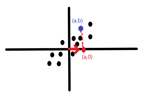
We can visualize this set of two dimensional data simply by plotting it as a set of points where is the entry in the first column and is the entry in the second column. To simplify things we’ll consider the data to be “standardized” ahead of time. If you don’t know what that means, don’t worry about it! It just makes the calculations simpler.

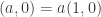
Additionally, let’s highlight one data point in particular and call it as we did with the matrix representation . This will help us see what PCA is doing to individual data points. Here’s how the graph of this data might look:

Right now, each data point is represented using the “standard basis vectors,” which are (1,0) and (0,1). This just means we can think of as :

If we reduce the dimension of the data set to a single dimension this really means we’ll only have one basis vector with which to write not just , but all of our data. We want the “best” basis vector for the job, meaning that we can use it to get pretty close to all of the data at the same time. If, for example, we only had access to the basis vector then the best approximation we could get of would be , meaning this is the closest multiple of to :

This is not a very good approximation of the data point . In fact every approximation of every data point using only the basis vector just comes from “projecting” onto the x-axis, which would be really good if all of the data was already near the x-axis! However, it’s not 😦

So what would a good approximation be? We’ve already hinted at it in the previous paragraph by using the word “near.” We want the transformed data to still be near the original data, so we should minimize the total amount of distance from the original data points. At the same time we want the transformed data to fall on a straight line so that a single basis vector can approximate all of the data. This is the same as projecting the data onto the “best fit line” by definition of the best fit line! It’s the line that is closest to all of the data at the same time:

To project the data onto the best fit line we just need some basic skills picked up in linear algebra. Scale the unit vector, which we call , pointing in the same direction as the best fit line by the dot product between the data point and ,

Thus the original data point is transformed into the data point: If we index all of the other data points: then we can write their transformed versions in the same way: . Again, this simply projects each data point onto the best fit line as pictured above. Thus each of these transformed points are approximations of the original data points with the added convenience that they can now be approximated pretty well by scalar multiples of the just the unit basis vector .

Additionally, since each of the approximations is just a scalar multiple of we can view the transformed data as just being the scalars: themselves. Visually we can picture this in the following way:

This reveals the dual way of thinking about what this transformation of the data does. The transformed data points are now just numbers living in one dimension, and they are all quite spaced apart! In fact, they are as spaced out as possible in the following sense. If we used any other unit vector besides the one pointing in the direction of the best fit line, the resulting numbers would be less spread out. The amount of spread for a given set of numbers can be measured in several ways, but we use “variance.” Thus, by dotting our data with the unit vector pointing in the direction of the best fit line, the transformed data has maximal variance. This viewpoint is the one we take when extending the ideas into higher dimensions.

Suppose now that we do not want to reduce dimension, and instead we want to look at our data in two dimensions, but from a different perspective. This means we need a second basis vector with which to express the data besides the “best” one from before: . What should our other basis vector be? Since we still want to have a basis it makes sense to use an orthogonal unit vector obeying the same kinds of properties as the first vector.

We want the vector to still maximize variance, while at the same time being orthogonal to . Since we are only dealing with two dimensional data, this does not leave us many options, we use the vector :

This projects the data to one dimension again, but this time by dotting with , the unit vector orthogonal to . By turning into both and we are really writing in terms of the basis vectors and which we can think about visually as:

In terms of matrices we are doing:

So the simple idea behind PCA is to find these “best” vectors and , and then dot them with the data to get transformed data. What are these “best” vectors? In two dimensions we saw that the unit vector pointing in the direction of the best fit line is the “best” because as a single basis vector, it’s the best at approximating all of the data at once by virtue of the best fit line minimizing the distance to all points. Then we noted this is equivalent to maximizing the variance of the transformed data. In higher dimensions it’s harder to visualize what’s going on, so we need to be more general and just think about if we have a matrix:

then we can project onto one dimension by doing matrix multiplication where:

and the result will be a matrix with only one column. This column is the transformed data and it’s one dimensional, so just a single column of numbers like before, written in terms of the basis vector c:

We want this resulting single column of data to have maximal variance. Recall that the variance of a bunch of numbers is given by averaging their square distance from the mean. Since we are working with standardized data the mean is 0 so the variance of is given by:

and we want this to be maximized. We can think of in a slightly different way, which you can check the by multiplying out the matrices:

The middle matrix, is an important one. It has variances of each of the columns of the original matrix X as diagonal entries. Meanwhile, the rest of the entries will be the “covariances” between any pair of columns, where in general the covariance between two standardized columns of data and is given by:

Name each column of , and the result is:

which is called the variance-covariance matrix of , or . In general this matrix has real entries and is symmetric because . We can now rephrase our goal. We want to find the vector c that maximizes:

Since is real symmetric we can decompose it as where has the “eigenvectors” of as columns, and:

has the corresponding eigenvalues as the diagonal entries and 0’s elsewhere. An additional nice property is that is an orthogonal matrix meaning that . Now we can show that is automatically a unit vector because is a unit vector:

Since and are both unit vectors this means that , which we are trying to maximize, must attain the same maximum as . This follows because and both range over all possible unit vectors, so that the two matrices range across the same sets of possible values. This new matrix is much easier to maximize though! Note that so that:

Now since because is a unit vector, this means that:

can be at most where is the largest eigenvalue of , which occurs when and the rest of the . Thus:

is maximal and equals when is the eigenvector corresponding to the largest eigenvalue, of the variance-covariance matrix. Therefore, to summarize, if you want to transform your data:

into such that the resulting data has maximal variance:

then you should use the eigenvector:

corresponding to the largest eigenvalue of:

and this is the “first principle component,” which is really the data projected onto one dimension using PCA. If you want to project the data to two dimensions, then you need another :

to help you get a second dimension. Following the same kind of logic, that is, wanting to maximize resulting variance, we choose to be the eigenvector corresponding to the second largest eigenvalue. This is because we want to have a basis with two vectors, so an additional constraint is that this next vector should be orthogonal to the previous vector.

In general the result of PCA is that the matrix gets transformed into the matrix whose columns are where is the ith eigenvector of ordered by size of corresponding eigenvalue. We rename these vectors because we can’t just call them all c:

Then, to reduce the dimension of X to from dimension n to dimension k we simply keep only the first k columns of Y:

We can then think about how much of the original total variance of the data from has been retained by using another nice property of matrices. Here we think of the total variance of the data in matrix as the sum of the variances in each of the columns of . This is exactly the same as the sum of the diagonals of the matrix :

The sum of the diagonals of a matrix has a name! It’s called the “trace” of the matrix. The trace happens to also equal the sum of the eigenvalues of the matrix, so we can say that the total variance of is . If we order the eigenvalues by size then decide to keep the first columns of the transformed matrix this means that the variances of the columns of will be and so the proportion of variance retained in the columns of is given by: .

The Return to Teaching in Person and Addressing Negative Comments

This semester we were back to teaching in person! I taught Calc 1, Calc 2, and Elementary Stats. I learned some valuable lessons, so I wanted to summarize them. I also received some negative comments and I wanted to take some time to address them directly. I do this to vent because it was very jarring. I’m accustomed to some negative stuff in my evaluations, and since those are private I don’t really comment on them publicly. This time, a few students disliked me enough to actually write about me on rate my professor!

How I set up my classes

Before the semester started I wanted to set up my classes in a way that would make their transition back to the classroom a bit easier. I assumed they probably struggled in the previous year, so I really wanted to simplify everything and give a lot of opportunities to get points back. In my calculus classes I decided to have weekly Quizzes that would account for 45% of the grade, and I decided to have no assigned homework. Instead, I posted daily sets of practice problems corresponding to every lecture, and the Quizzes would just be based on those problems. In fact, sometimes I didn’t even change the problems!

Then I made the Quizzes open note. Ideally, a student would do the practice problems and be able to use their work to do the Quizzes very comfortably. Then I allowed students to reattempt Quizzes as many times as they could fit in before the corresponding midterm, i.e. Quizzes 1-5 had to be turned in before Midterm 1 and Quizzes 6-10 before Midterm 2. I graded each problem as either correct, needs to be fixed, or needs to be redone.

If I wrote “fix” this meant that the student made decent progress on the problem, but it was still a ways off. The student could then take the time to fix their work and resubmit it for full credit. If I wrote “new” this meant that the student made little or no progress on the problem, and that they would need to come to my office and do a new, but similar problem, to get the credit.

Each Midterm was then 10% and the Final was 30 % and could replace the lower midterm score. The last 5% comes from daily problems where they just do a quick example at the end of each class for a basic check for understanding.

What could go wrong?

When I set this system up I understood the common risks of not having assigned homework and having a redo system set up. That is, students may not do the practice problems if they are not due for points, even though the Quizzes will be based on them. Also, students may wait until the last second to reattempt problems and so they really only get a second try. They might not study for the Quizzes because they think they can just easily get the points back later.

Many a student has succumb to the forbidden fruit of “I can just get points back later, so I’ll not worry about it right now” only to find it’s week 5, they don’t know anything from weeks 1-5, they need to reattempt a bunch of problems, and they need to study for the midterm, and they’ve never attempted a single practice problem. I tried to warn them about this trap over and over! It also seems like explaining concepts well makes the situation worse because after each class they feel like they understand what’s going on and think they don’t need to do the practice problems. I shouted endlessly into the void to try to get them to do the practice problems, but few listened. I know this because I discovered I can actually check which students have opened my files!

Unexpected flaws

There was one risk that I did not foresee, perhaps because I was a bit too naïve.

This system, which I set up to preemptively be really nice and helpful, would come to be seen as standard. This meant that students would often ask for even more opportunities or more advantages, and be very upset when I said no, as if I had not already built a free 45% into the grade from the start! In fact, I suspect that if I did not build these advantages into my class from the start, and instead I said at the last second: “by the way you can redo Quizzes” then I would have been hailed as the nice professor who gives opportunities instead of the mean professor that says no to everything.

Here are some examples of how I became the mean professor:

1) Exhibit A from Rate my Professor:

Now I would like to address this comment from my perspective.

Student would need to reattempt a Quiz problem in my office. They would come unprepared and without having bothered to learn the original problem that they got wrong. Then, they would ask me to help them with the new Quiz problem and I would say that I cannot because it’s a Quiz, but I would be happy to help them with the previous Quiz problem or the similar practice problems (that they never attempted) in order to prepare them to do the new Quiz problem on their own. Student instead goes back to attempting the new Quiz problem in a huff and decides that I never help when they ask for help.

In this scenario the fact that they can even redo the Quiz has been completely forgotten as the nicety, and I’m now mean because I will not help them literally do the Quiz as they do it. Apparently, I also came across as disrespectful when saying no. That may be true as I got more and more annoyed at this pattern of not asking me for help learning, but instead asking me for help getting points.

I would take this comment more seriously if not for the last sentence being a complete fabrication. I absolutely mentioned that the Final exam will naturally be harder as it’s cumulative, but that I will make each individual problem be easier than the previous iterations to make up for this. The comment also reeks of entitlement. I read it as “you should just give everyone free points instead of opportunities for free points.”


2) UPDATE: Apparently this review was deleted from the website! I’m not sure how that happened, but in any case I’ll leave this part up. Exhibit B from Rate my Professor:

Grading not making sense:

Student turns in gibberish work with a magically correct final answer and asks why I wrote “fix.” Student gets annoyed that he has to have correct work, or at least not gibberish, because correct work is part of the answer. Even though this happened exactly one time, student now believes I’m out to get him with my mean grading and that I just grade everything as incorrect even though everything he’s ever done has been correct.

The easy way to remedy the situation would have been to ask me for help doing the similar practice problems, but unfortunately this did not happen. I suspect this comment was made by the student who missed, or was 10-40 minutes late, to every single class, which will certainly create giant gaps in understanding and cause a student to write gibberish work.

Takes forever to grade:

Student turns in Quiz 1-5 fixes and reattempts all at once the week before they are due. Then asks me every single day if I’ve graded them yet, so he can try again. Since several other people have done the same thing in all three of my classes I tell him that no I cannot possibly grade them all this fast so I probably won’t get them done before the midterm. From his perspective I am grading very slowly, even though, without fail, I returned the Quizzes within 2 days of the first attempt every single time, so that they could have lot’s of chances. If he had reattempted the earlier Quizzes more quickly, then I would have had time to grade more reattempts.

Since he was out of time, I suggest taking the problems back and making sure they are correct before turning them in, but he just wants me to grade them really fast instead so he knows if he should bother trying again. I also suggest trying to redo the earlier Quizzes more quickly next time so that he will definitely get more tries. Student does not do this for Quizzes 6-10 and instead also turns them all in right before the second Midterm, and once again expects me to have superhuman grading speed.

Conclusion

I want to emphasize that I’m not trying to pick on the students who wrote these comments. Most likely these kinds of thoughts were held by multiple people in the class. Students are young and they procrastinate a lot, and the system I created was meant to give them opportunities, but I think instead it made them procrastinate more than they normally do. Then they found out the hard way that you cannot just learn everything in a math class at the last second. I worried this would happen, but I tried anyway.

Most of the time negative comments are not helpful, as I sort of already know what went wrong or how to improve. In this case, negative comments have actually given me the following realization.

Instead of preemptively building opportunities into your syllabus, casually throw them out there during the semester. You will seem like a hero. Otherwise, you run the risk of being the terrible and mean professor.

Teaching Differential Equations Online, in a block format

This spring I was fortunate enough to teach differential equations! As I’ve mentioned in previous posts, we’ve been in a block system this year. This meant that the class was to be taught in only 6 weeks!

I’ve taught a lower division differential equations class before as a graduate student. In fact, I taught it two summers in a row. This class sort of lies between a lower division and upper division differential equations class because it’s meant for a semester, and has no proof knowledge prerequisite. This was nice because it meant I could start from the beginning and teach about a lot of things I’ve already taught, but then I could eventually move into areas that I’ve never taught or learned before.

Due to time constraints I cut out some of the magical seeming techniques one often encounters in this class. Specifically, I did not teach how to solve Bernoulli equations or exact equations. I wanted to get to the more interesting stuff at the end of the class. It worked out so well that I think even during a full semester I would still cut these two things out. All the really fun stuff in this class happens toward the end anyway.

My only regret is not having time to teach any numerical techniques.

In general I really loved explaining this stuff and my class really seemed to enjoy it too. We had a class “Discord” where students could quickly communicate with each other and me. We could laugh and joke around as well as discuss the math in the class. They sometimes cried over math too though. Woops!

I often enjoyed explaining random math things not in the class by writing little blurbs and drawing pictures in the Discord.

I’m looking forward to the evaluations. Hopefully they remembered to write something!

For grades I decided to be extremely generous as I have been with all my classes during the pandemic. I did add a new bit that I think I’ll keep in the future.

First, their grades were based on 5 Quizzes. Questions were typically worth 5 points and the new thing I did was, if they got a 3 or 4 on a problem they could fix it up and resubmit it for full credit. The idea being that if they only made minor mistakes they demonstrated near mastery knowledge, but I still wanted them to fix things up to get the full points. If they got below the threshold then they would have to do a makeup problem instead, which would be slightly different and appear on the next Quiz. They could keep retrying different variations of old problems on each Quiz, but eventually due to time constraints I had to allow them to do makeup problems on their own time instead of in a timed Quiz setting.

I liked this a lot, but it could use some fine-tuning. Not that I would ever complain about giving out too many A’s… but yeah I had A LOT of A’s, which is probably not indicative of actual understanding.

Once again I kept things simple when it came to imparting knowledge: video lectures followed by corresponding lecture problems that I would help them with during Zoom meetings. I’ll be adding the playlist for videos as well as the corresponding lecture problems to my other page! I think anyone whose taken Calculus could follow this course.

The thing I enjoyed most about this class was finally getting to learn about Fourier series. I’ve never bothered to learn about them, but I knew they were secretly really cool. They did not disappoint!


I’ll leave you with this word problem that appeared on one of my Quizzes. It features my unique art style:

Teaching Abstract Thinking in a Block Format

I just finished up teaching “Abstract Thinking.” Before finishing up the grades I thought I would relax by writing things up.

This class is often titled “Introduction to Proofs,” but I really like our title because it sounds a lot smarter. This was the first time I’ve taught this class and it was just as fun as I had always hoped. This despite the fact that it was completely online says a lot about how interesting this class is! In this post I’ll talk about my experience.

Content of the Class
The content is the most interesting aspect of this course so it has to come first! In this class a student transitions from learning how to do things to learning how to prove things. For example, many people can do this: 2+4=??, as well as infinitely many other versions of this question. A smaller number of people may notice patterns like, whenever I add two even numbers up the result is an even number. 2+4=6, 10+20=30, 16+6=22. This seems to check out! And finally, math people will go a little bit further and say “I can prove this is always the case!” by specifically defining what an “even number” really is, abstractly. Hence the name of the class.

An even number is a number which can be written as two times another number. This is where math symbols come in handy! It’s more useful to say: An even number is a number x, which can be written as x=2n, where n is another number.

Now, math people will be even more specific than this, but I don’t want to hassle over minor details because this will lose readers!

Once you have this definition you can think about, what happens if I add up two even numbers: x+y=???

Well, I know that x is two times a number so I’ll say x=2n. I also know that y is two times a number so I’ll say y=2m. This means x+y=2n+2m. Why is this an even number? It needs to be 2 times a number, so is it that? Yes, because I can write 2n+2m=2(n+m) as long as I remember some algebra! Writing this argument up in a nice way creates a formal “proof” of a formal “statement” that says: If I add up two even numbers, the result will be an even number. Math people prove formal “statements” like this for a living.

My goal was to get students to start writing proofs as soon as humanly possible. Sometimes instructors run circles around the true purpose of the class before really going for it. By the time you start proving things you’ve done way too many other things as background information. Statements, logical operators, truth tables, sets and notation! It’s all fun and interesting stuff to talk about, but unfortunately to a complete math newb it’s all a distraction. They are not yet advanced enough to appreciate the justification that truth tables provide, nor do they appreciate logical operators without having done a bunch of proofs that secretly involve those logical operators first. Before you can appreciate the complexities of the most appetizing cookie recipe of all time you just need to eat a few first.

So my plan was to tell students what a “statement” was; it’s a sentence that is either true or false. I gave many examples, like “My car is red,” which happens to be a true statement. Non-examples like, “My car is cool,” which is an opinion that is neither true nor false, are equally as important as examples! After this I explained that a mathematician’s purpose is to prove true statements true and false statements false. Then I narrowed our focus by specifically only dealing with “conditional statements.” These are statements of the form: If _____ then ______. Then BAM! Time to prove some of these bad boys.

If you spend too much time on logical operators and truth tables so that you can justify proofs and various techniques then you’ll never have time to practice! I think it is almost completely clear how to prove something like:

If x and y are even, then x+y is even.

once you have been walked through an example or two, but you can make it seem a lot more intense by first explaining in general how one should “prove a conditional statement where the hypothesis has a conjunction of two predicates.” Just by introducing conditional statements, and the definitions of even and odd, you can get them to start practicing writing a lot of proofs! You can even sneak in “and” statements and “or” statements without them even realizing it! In retrospect and with more time to spare I would have made them spend a little more time on this stuff before moving on to formally talking about logical operators.

One way I wanted to veer of the usual path in this class is to spend very little time on truth tables. These show up pretty quickly because once you introduce “and” and “or” you are forced into talking about truth tables! These truly elegant gizmos are wonderful if you already understand a lot of math, but if you are a student learning to prove things they are a crutch. Here’s what they think as they see a truth table problem on an exam or homework: “Thank god some calculations I can do for free points instead of these damn proofs!” In my class there were no such resting points! You shall not truth table your way into a C in my class. I made the professory decision to use truth tables as sparingly as possible. I only used them as justification for proof techniques and I only made them calculate a few very small truth tables. Just the ones that create interesting relationships between logical operators because those are actually interesting on their own. Never did I make them calculate a big bad truth table.

To create more interesting examples of statements we next need more interesting definitions! Even and odd numbers can only take you so far. The next definition is the definition of “divides,” which sounds very strange to people that know how to do division. At this point I took another different path by skipping something very standard. I decided not to talk about “congruence” or “modular arithmetic.” My reasoning was that, first of all they will start this stuff from scratch in a Number Theory course anyway, and second it gives too many calculationy things to do. I really wanted them to focus on proofs and so right after defining “divides” we moved into other proof techniques which combined with the definition of divides, gives a lot of proofs to practice! After this was learning about induction, which again works great with the definition of divides!

Next I moved into Set Theory. All of the proofs they did before involved essentially showing facts about numbers. It’s a good starting place, but another big point of this course is to make them realize that math is not just about numbers. Set Theory creates a wonderful playground for learning how to prove things about gadgets they’ve never dealt with! They really have to learn how to deal with definitions based on exactly what the definitions say. Without intuition and background familiarity like they have for even and odd numbers, they have to keep looking at the definitions to prove things. This is nice because it throws them into the deep end of the pool, but with some floaties still on (me). There’s a lot to say about Set Theory in this class, but it’s all pretty standard from here so I’ll jump to what I did differently towards the end.

In my last two lectures I was able to talk about operations on sets and functions preserving operations. The idea here is that operations we are all familiar with like “plus” and “times” should really be thought of as ways to combine two things of a certain kind into another thing of that same kind. For example, “plus” turns 3 and 5 into 3+5, or 8. Two numbers turn into another number. A first grader would probably say: 3+5=8. But a highly skilled mathematician might say: +(3,5)=8. Once you learn some set theory you can write fancy things like this too!

Once you learn about operations you can try to think about operations that are less familiar and boring. Yes, we know how to turn two numbers into another number, but there are operations that turn two not-numbers into another not-number! Then you can try to think about similarities and differences between these other operations and “plus.” For example you might know that 3+5=5+3 and that this switcheroo always works for addition of numbers! However this rule is not always a given in other situations.

In the end I was able to summarize that math people like to “study sets equipped with operations.” Then there are a few main questions we can ask. 1) What are all the sets equipped with operations obeying the same rules? 2) What are additional properties of these sets with operations? When are two “the same?” What does “the same” mean?

In fact, I really wanted to do a preview of other classes at the end of this class, but only managed to have time for Abstract Algebra. Ideally I would have a “fun” end week where I could do similar introductions to other courses.

How I Ran the Class

Due to the current pandemic I taught this class virtually. As far as I can tell using lecture videos is the best way to teach online. Live lectures are just too risky. Certainly for precalculus type classes lecture videos work very well. Students can watch and rewind when they get stuck or accidentally fall asleep, unlike in class where if they fall asleep they are permanently behind. I was a little worried that videos would not work so well in this class because it’s a very different type of class. Oh, and not only was this class online, but it was also turned into a 7-week block course instead of a full semester course!

Despite the odds being stacked against me I went ahead and made lecture videos. I think I made about 15 lecture videos before the course started. I made 20 if you count the first 5 crappy ones that I made, but then redid.

My plan was for students to watch lecture videos on their own time, while during the designated course time they would work on corresponding lecture problems. These meetings were not mandatory. For the first few weeks I would break the students up into groups to work on these problems. As I suspected might happen, attendance began to dwindle and students would just silently work alone in the breakout rooms. So I ended the breakout rooms and then students would occasionally ask me for help, but still mostly stay in silence and as an empty void on Zoom. During these meetings I would work on solutions to the lecture problems in an overleaf file that they could see updated live. After the meeting I would post the complete solutions.

Since the course was 7 weeks long it was jam packed. They had to watch a video almost every single night and then work on corresponding problems every single day. Their only respite was before a Quiz. I broke the material up into 3 Quizzes, which accounted for their entire grade. I decided that homework would be impossible to keep up with in terms of grading so I never graded any of their work on the lecture problems. This turned out to be a very good idea because towards the end of the block I could barely keep up with making a new video each night. This is because I had another course to teach at the same time.

Grading

I really liked the grading method I used in my upper division linear algebra course so I decided to use it again here from the beginning. Each Quiz consisted only of proofs, since the point of this class is to learn how to prove things. 70% of each Quiz was “all or nothing” meaning you either get all the points or you get none, depending on if your proofs made sense. Minor mistakes do not count against you, but you also cannot build up pity points by writing gibberish. The proofs corresponding to these points were supposed to be “basic” in that to succeed in the future you at least need to be able to do these level of proofs. The other 30% of each Quiz consisted of tougher proofs that students could earn partial credit on by starting them correctly, making progress, and writing true things.

Linear Algebra Done Okay.

I just finished teaching a course in upper division linear algebra. I decided to put down my thoughts because I happen to have a phone interview tomorrow and I thought this might help me think about the kind of stuff I might say. This post will consist of two parts.

How to begin a class on upper division linear algebra

This was the first time I’ve taught a “proof based” course. My plan was to mesh the two books: “Linear Algebra Done Right” and “Linear Algebra Done Wrong.” So I called my class “Linear Algebra Done Okay.” To start the class I did my usual ritual. That is, I spent large chunks of my summer writing lectures. In total I must have rewritten the first lecture 5 or 6 times. Then I wrote approximately 3 weeks of lectures. Then, as is tradition, I threw it all out because it was garbage. Then I wrote the lectures twice more until I was happy. If I recall correctly I managed to write enough material for about 7 weeks of class.

I found it hardest to explain the material at the start of the class so that’s what I want to talk about.

It seems like most books either jump into vector spaces too quickly or finally introduce the holy grail after an agonizing amount of time spent in and . They either define fields and vector spaces immediately or take a chapter to draw lots of nice pictures. Then they point out some neat little axioms that just so happen to be true in . But this always bothers me because the axioms are just a bunch of obviously true rules to students because the book just spent tons of energy on an example where they are true. So then you say “viola these rules are great so we’ll just write ’em down without any reference to numbers.” But the rules are not weird enough to then give examples of why you would want to write the rules down. So the students just think why the hell have I written the rules down a second time or third time? They don’t get the point of axioms generalizing the rules we observe because vector spaces are too nice.

In order to appreciate rules you have to get into a little trouble first ;). So I decided the following approach would be the best.

I think the best way to do it is to talk about sets and operations. They’ve taken the introduction to proof class, but likely are not that comfortable with sets yet, or proofs for that matter. So ideally this would connect new information with old information and give them some minor things to prove for practice. Formally defining operations as specific kinds of functions lets you eventually define a field with some proper motivation. Otherwise it seems like you just say “here are some field axioms, oh by the way there are other fields besides and .”

I prefer to slowly build up to fields from monoids, groups, and rings, so you have examples where you don’t just get to use every rule you are accustomed to from 14 years of studying numbers. You don’t need to investigate monoids, groups, and rings in detail either. In particular I think working with nice picture-esque examples of monoids and groups serves to adequately convince them that there are cool such thingies and therefore studying these thingies might be a good idea. Then the motivation is that math people like to study sets with operations obeying rules. Finally fields come in as the sort of final and “best” algebraic gizmo because you get to use every rule you want to use.

All of what I mentioned is ideal. Instead I rushed through this stuff in a single day because the books made me feel like I just needed to say what fields were as fast as possible so I could say what they really want me to say: “fields are where scalars come from, but we don’t study them in this class anyway so don’t worry too much.” I know that when teaching set theory as an introduction to proof class most instructors don’t talk about operations, which I feel is something that really should be done. Down with truth tables! Spend some time talking about operations!

In any case I managed to define vector spaces as sets with two operations such that blahdy blah. However, proving something is a vector space has got to be the absolute worst and most tedious thing to prove. In any case this is about as much as I want to say about the material itself. I felt that I presented the rest of the material very well.

How to ensure that students can write a basic proof.

Instead I want to talk about how I adjusted my expectations and my goals for the students. I had already planned to constantly explain how proofs work, but I ended up having to do a lot of extra and different things. Whenever I presented a proof I was sure to discuss and emphasize the following points.

1) Write down what you are given and what you want to show.
2) Elaborate on what you are assuming. That is, write down what it is you are actually assuming. Do this several more times until it’s completely clear what you are really assuming.
3) Elaborate on what you are trying to show. That is, write down what it is you are actually showing. Do this several more times until it’s completely clear what you are really showing.
4) Know how to start showing what it is you want to show. This is where students struggle a lot.

Students struggle a lot in starting proofs. The biggest example is getting them to show that some vectors are linearly independent. This one in particular is difficult for them because they don’t yet understand the if/then nature of definitions.

Very quickly I realized that there were roughly 4 students that came into the class with the ability to write down a proof. The other 12 had no clue despite all passing the introduction to proofs course. In the first couple of homeworks they would either write gibberish or perfect answers, which were obviously copied from somewhere. My usual methods for teaching proofs were not enough, but I also couldn’t slow down too much because I had these 4 strong students who were in need of more and more material.

My first remedy was to create some “how to” worksheets. I compiled a list of definitions and made a worksheet called “Proof Techniques.” For each definition I wrote something like:

To show that a set of vectors is linearly independent you LET
and then SHOW that .

If you are given that the set of vectors is linearly independent then IF
shows up somewhere then as a result you may CONCLUDE that .

I also made a worksheet detailing how to approach a proof or problem that you don’t know how to just do. I thought this was necessary because sometimes students felt like if they didn’t know how to just see it and do it immediately that the solution was to give up and google it or give up and ask me. They don’t realize that you are suppose to struggle, but even worse they don’t know how to struggle in a successful way.

However, I don’t think my additional materials helped all that much at first. Partly because they didn’t use these materials and didn’t take it seriously enough. For you see I made the fatal mistake of allowing students to make up any and all homework points that I so unfairly stole from them. They merely had to redo and present the proof in front of me. To aid them in this I even wrote up solutions to all of my homeworks. Instead of using my solutions to learn how proofs work they just memorized the proofs. So whenever they made a typo and I asked even the most minor question they had no clue what was going on.

My first midterm was very standard. Write down some definitions, do a medium proof, do a hard proof, do some true/false. Here they can build up enough “pity points” where pity can either mean that I am showing pity or that they’ve given me a pitiful attempt at an answer. These pity points and the free homework makeup points were leading me to horrible and unavoidable conclusion. My students still couldn’t write a basic proof following from a definition, but they were going to pass my proof based course.

Due to this I had no choice but to take some drastic measures in what I asked them to do on the next midterm and final. I had to be sure they could prove something so my second midterm simply consisted of five proofs. Three of the proofs were extremely straightforward from definitions. For example: show ___ is a subspace, where as long as you knew how to start a subspace proof and how to write what it means for vectors to be in the set then you don’t have to do any tricks to make the proof happen.

These simple proofs were weighted such that if you could do them you would pass. To ensure that proving something was the bar for them I graded these “easy” proofs in an all or nothing way. If you “got it” you got all the points even if you made minor errors or left details out. If not, you got 0 points. This ensured that if you focused on mastering the basics you were guaranteed to pass. The two harder proofs were graded in a more standard way, so if you could at least start them and write down relevant information then you would get a 75 (if you also got the easy ones).

On the midterm this failed, sort of, in that a large number of students barely got one of the three “correct” in that they did just enough to get me to give them all of the points instead of none of the points.

The final went much better. I gave them 9 proofs where 5 were easy and weighted appropriately. A large chunk of students were able to do all 5 at the level to get all the points.

My First Year as a Professor (Fall Semester)

This year I worked as a visiting assistant professor at Whittier College. It’s a small private liberal arts college in Whittier. My year consisted of teaching, teaching, and more teaching, not that I’m complaining about it because I love it, but it was far more than I was used to. Throughout graduate school I was able to slowly increase the number of hours in which I could do productive work per day, from about 1 to 6. During graduate school I spent most of my productive hours doing research.

This year I spent most of those precious productive hours teaching, thinking about teaching, helping students, or grading. Again, I’m not complaining; I really do love it. I managed to attend the weekly Network Theory seminars back at UC Riverside, but that’s not research. Quietly listening to math is not doing math, but it did help me keep the stuff I already know from leaking out of my brain. And I don’t want to lie to myself, I actually went for the people and the beer.

This post exists to detail my first experience as a professor.

In the Fall semester I taught two sections of lower division statistics and one section of differential calculus. First I’ll talk about teaching stats, since anyone reading this will probably have taught calculus themselves many times. Stats is quite a different beast and worth talking about.

When I taught differential equations in the before time I wrote about 5 weeks worth of notes and homework before the class even began. Yes I knew the material already, but writing down how I would actually teach it is one reason the class went very well. Anyone who teaches will tell you that teaching something the first time is the hardest. So I skipped that experience by writing out lectures for nearly the entire course. I think I rewrote my first lecture about 5 times. The final time being after I had written 4 weeks of material and decided to just start over again.

Basically, when I taught differential equations for the first time I was actually teaching it for the second or third time.

However, I was unable to do this for stats because I didn’t really know what the class was about until about a week before it started. I had no experience as a teaching assistant for stats and I hadn’t seen the material since high school. My first lecture went about as well as I expected, i.e. like as bad as a really bad simile, like this one. I felt as if I were giving my first ever math talk all over again. Where, although I know I’m saying a bunch of technically correct things, I have no clue what I’m talking about.

My two sections of stats were offset, one was MWF and the other TTh. My MWF class did not care for me, but my TTh thought I was great. Here’s why!

Every Monday I would give a terrible lecture, then I would go home and write down everything the way it should have been said. Then on Tuesday I would give a clear and helpful lecture followed by some extra time to work on problems or homework. Rinse and repeat for 13 weeks and you’ll read in my evaluations from one class that I sucked, and the other that I was amazing. I tried to make it better by scanning my better notes for my MWF class, but as it turns out students do not read anything at home.

In the end I really enjoyed teaching stats because I learned some new basic math at a deep level. I was going to say more about this, but there’s just too much. I’ll need to write another post just to talk about lower division stats. Moving right along to calculus!

I was able to prepare very far in advance for calculus and so it went very smoothly. Also, I just know it very well and I’ve taught it many times. Some days I looked at what the topic was and freely generated my lecture, and those were some of my best lectures because it meant I was more interactive and interesting. Just like in differential equations I wrote my own homework and had lots of walk-through problems. My class seemed to like it by the end, although at first it was a shock to them. I think I did a very good job in terms of explaining the material and I think the homework was helpful.

The first midterm inevitably crushed my spirits as it crushed their grades. They did horribly on what I thought was a midterm for little babies. I went to class that day thinking, “shit I made this thing too easy.” I had given them a review guide too, where I essentially pointed out exactly what problems I would be asking them to solve. If I remember correctly one student finished in about 25 minutes (because yes it was actually very easy), while the rest struggled to finish on time.

At first I blamed myself and felt gutted. Where did I go wrong? How could they do this poorly? It was as bad as a calc class taught by a visiting professor at UCR whose never taught before. Here I thought I was some amazing explainer, but clearly I was terrible. Nobody knew anything at all!

I looked over the exam again and it was as pathetically easy as I thought it was. That’s why one student was able to get 100% and finish in 25 minutes. I felt bad for him because there was absolutely nothing challenging about it.

I realized that they just did not study.

Or perhaps they did study, I thought, but they didn’t know how to study efficiently. Maybe they didn’t know what it meant to study; they need to study studying! Perhaps they just glanced at topics and did not heed my study instructions, where I made what it takes to do well very clear. So I tried to pester them about working harder, asking me questions, practicing until you’re perfect, etc. For the second midterm I made actual review questions, instead of just a very specific review guide. I was basically gifting them the next exam.

Foolishly I thought, “this time surely!” I walked in thinking once again, “oh god I’ve made it too easy!”

Again one student finished with a perfect score in 25 minutes. A couple students did slightly better, but most remained the same or actually did worse. I continued my spiral. I loathed myself.

I had thought very highly of my teaching ability for so so long. I questioned myself a lot throughout this semester. Was I ever actually good at this? Was I just dreaming at UCR? Were people just pretending I was good at teaching to be nice, but secretly I was the worst teacher? Was I just all talk? Maybe I convinced myself I was good at it, but I never actually was?

It’s the same story for the final, but someone asked me a question during the final which finally allowed me to move on from blaming myself. Towards the end of the semester we learned about some very basic differential equations, the separable ones. I told them they would need to solve one on the final. I put an example on the final exam review guide. I had 2 in class days of review and posted solutions to the review problems!

During the final a student raised their hand, pointed to a problem and says “what does this mean, solve the differential equation?”

So then I realized, they don’t study and sometimes there’s nothing I can do about it.

I just try to be approachable and make sure they know I want to help them. Most won’t take me up on the offer to help them succeed, and that’s okay. A lot of them are just kids and don’t take things seriously yet. I’m content with helping just the one or two people in each class that want the help. If I can get them to improve and enjoy mathematics then I’ve made a positive impact.

In the next part I’ll talk about my second semester.

My Experience Teaching Differential Equations

This summer I taught lower division differential equations. The purpose of this post is to share my experiences and recommendations for teaching mathematics with differential equations as an example.

In summary I emulated the things that I’ve seen John Baez do in classes I’ve taken from him. I consider the most important lesson I learned to be the way in which he does homework. Briefly, homework should be like a story that leads the reader into learning something new. I’ve attached my homework assignments at the bottom of the page for anybody who wants to see how it works without having to read my entire post where I’ll go into more detail.

I had been a teaching assistant for this class so I knew a little bit about what troubled students and about what I should cover. Additionally I had some discussions with another graduate student, Andrew Walker, who taught this course the previous summer. From our conversations and my personal experience I believe the following things to be useful notes.

1) Instructors artificially increase the difficulty of this class by making problems that require difficult integration techniques.

In my opinion the point of a basic differential equations class is to learn how to solve some differential equations, not how to solve difficult integrals. Difficulty can be increased in other more productive ways that deal with concepts strictly having to do with differential equations. Students get so bogged down that they leave the class without ever grasping what they were supposed to. It seems like many students finish without understanding what it means to solve a differential equation, what a solution is, or even what a differential equation is.

The solution to this issue is simple- when integrals are necessary for solving a technique make sure problems being done have easy integrals. It’s a bit painstaking to create problems which satisfy this condition, but I believe the payoff is absolutely worth it. (Note: Rarely tough integrals are unavoidable!).

2) Students only write down what you write down.
Even the best students can’t write as fast as someone can talk. Math instructors are too often guilty of haphazardly writing down concepts while verbally explaining important points or sloppily writing down a solution without a single word on the board. The verbal explanation can be enlightening and perfect, but if the students can’t copy it down then they probably won’t remember it!

While teaching differential equations I wrote down every single concept that I wanted students to understand in complete sentences and in complete detail. I wrote down every single example I did as complete thoughts and sentences which brings me to the next point.

3) Writing complete sentences to explain math is a must.
It’s best to illustrate this with an example. I may eventually upload my notes, but for now the following will suffice. Suppose we had a question that said, “Solve the differential equation ”

Many professors will teach this in the following way. They will say (but not write) that this differential equation is separable and explain things (verbally) about separable equations while simply writing on the board-

The student will then write the same 4 lines in their notes. Instead the instructor should write the following on the board-

Since,

is a separable equation, we can “multiply” to get

then we can integrate both sides to get

so that

This problem is simple so it’s possible a student can have a perfect understanding of what happened without the words, but difficulty increases it becomes more necessary to write complete thoughts and sentences so you may as well make it a habit during the easier topics.

Writing out problems like this serves a few purposes-

-By doing this enough times they come to understand mathematics is not just lists of equations. It’s about presenting something true in a very logical way that flows from a clear beginning to a clear end. They work the same way sentences do. Sure I could read a sentence with a bunch of things missing and get the gist of it, but whoever wrote it doesn’t really understand how sentences are used to express their ideas. Getting the final answer correct is much less important than having an understanding of the concepts!

-When problems are more complex students have notes that make enough sense to be useful. Words as simple as “since, then, thus, if” etc. increase understanding by a huge amount because the notes become readable. When looking back at notes they can easily follow along from start to finish instead of just seeing a jumbled mess of equations. The reality is that most will never open a textbook so this is their textbook.

-When they do problems on homework, quizzes, and tests, their solutions look much better because they start to solve problems in the same logical way. Their thoughts are clearly expressed. The lack of complete thoughts being taught to them from elementary school onward is evident in the work they turn in. It looks exactly like what they are told to do. That is, write down messes of equations that make no sense on their own and then a box around some final answer.

Besides writing nice details one should also reiterate additional details (like context) verbally while writing down the nice solutions, but whatever the additional details are should have been written down somewhere earlier when the concepts were being taught. The verbal repetition is just there to nail the ideas (which had already been written down!) into their head.

4) Assign written homework which acts like a story.

Traditionally, instructors will teach a section and assign a huge amount of problems which require the student to do the same thing over and over that they learned in the section. The idea is to get some process stuck in their heads.

The problem here is that different students need different amounts of problems until things click. Thus assigning a certain fixed amount is usually very annoying for students. The ones who already get it will be annoyed that they have to keep doing something that know how to do (over and over and over). Often they’ll not really know how to do it and just keep doing problems incorrectly which creates a bad habit! The ones who don’t get it will be frustrated that they can’t even start the assignment and still have so many more problems left to do.

It’s pointless because once you can do a few problems in a section that usually means you can do all of them.

I’ll try to explain my solution to this issue, but it’s better to see an example in the links at the bottom.

Assignments should remind students about what they’ve been doing in class with a brief explanation. Questions should lead students through the step by step inner workings of solving a problem without telling them too much. After they’ve gone through questions the assignment should explain to them what they just did and how it relates to other things they know.

This type of homework is more engaging and interesting without being tedious and repetitive. Unfortunately though repetition is also necessary at some point.  For this reason I also added some practice problems which are not required to be turned. My hope is without the burden of a due date the problems will seem easier. I also asked the teaching assistant to go over these during the discussion section in class to give them more help with the boring repetition.

I believe using the discussion section like this was very helpful, but I realize not all people have this at their schools. Speaking of discussion sections, I had them do 1 question quizzes at the end of discussion sections in order to force attendance. They were supposed to be similar to practice problems that the teaching assistant went over, but also way easier. The students knew it was coming so hopefully would pay attention to the practice problems and then be able to do a simple problem.

Finally, here are all of the assignments that I wrote. They work better with my specific notes because they tie into things that I did in class, but my notes probably won’t ever be typed up.

It’s possible that there are typos which went unfixed and I’m sure things could be explained better by someone more experienced. Additionally I would have liked to cover more topics, but it was my first time running a class so I didn’t have a good sense of how much time I had to work with.

If you are interested I can send you the latex files.

homework-1

homework-2

homework-3

homework-4

homework-5

homework-6

homework-7

homework-8

homework-9

homework-10

Category Theory for the Working non-Mathematician 2

Last time I talked about the very basics of Category Theory, objects and morphisms and what exactly a Category consisted of. If nothing else sticks just remember that categories consist things (objects) and ways to go between things (morphisms) where you always have the ability to go from something to itself by doing nothing and you can go from thing to thing to thing via arrows composed together having a common middle object. The next step is to figure out how to go between two different categories. At the moment our view of the world is like a human stuck on the earth. There are places on earth and there are ways that we can go from place to place (routes) and we can compose our traveling methods to get from one place to another and then to another. So a category is much like a planet. However humans are curious. We look up at the stars and we want to venture to other planets. We are also very fragile creatures and we can’t just go to to any planet all willy nilly, we have to go there in a very specific way so that we don’t die. Not only that but the planet we go to has to have similar features to earth, so that again we don’t die. I know how earth looks and so the best way to survive is to correspond this new planet to the one I already know. This very restrictive way of going from one planet to another is similar to the nature of going from one category to another.

Let’s think about what it would mean to go from a category C to a category D. We start out in C, and there is some set of objects. Well D also has objects so the most logical thing to do is to have something in D correspond to something in C. The mathy way to write this is that for any object X in C, there is an object F(X) in D. Simple, elegant, no restrictions. Now, there are also morphisms (ways to go between objects) living in the category C and D. Any morphism in C goes between two objects in C and I’ve already said that the objects in C MUST be associated to some objects in D. The most logical thing to do once again would be to associate a given morphism from X to Y in C to a morphism between F(X) and F(Y) over in the category D. This part is a bit trickier because I want the morphism in C to be associated to the morphism in D in a way that makes sense. If I have a way to go from California to New York and then I go to Earth 2.0 discover California 2.0 and New York 2.0 then I’m going to want the way to go between the originals to correspond to the way to go between the new ones rather than some completely different route.

How is this going to work? First of all we need better notation. We are going to start calling our space travel from Earth to Earth 2.0, a functor. A functor is a map from the category C to the category D that does the following. For any object X in C, there is an object F(X) in D. For any morphism between objects X,Y in C, there is a corresponding morphism 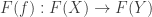which obey some rules to be explained later. For now just see how this functor is taking objects to CORRESPONDING objects in D, and paths between objects to paths between CORRESPONDING objects in D. What other rules do I need? Well if you will recall from the previous article, a category is not just objects and morphisms. It had some special rules about these things. Remember that for any object X in a category C there has to be at least this one special morphism; the identity morphism which was like taking the path from X to X by not moving. In the current analogy, I can go from California to California by doing nothing at all. Since C and D are both categories, they both have these special “do nothing” paths and so logically it would be best if we took the one from C and sent it to the one in D. So our first condition for the functor F is that . This is merely saying that F takes in the identity morphism from X to X, and sends it to the identity morphism from F(X) to F(X), which is the object in D that corresponded to X in C via the functor.

The last condition we need involves the other property that was forced upon a category in the previous post. In any category we had to be able to put two morphisms together, i.e. compose two morphisms and to make one longer morphism . So let’s see how this works with our functor going from one category to another. First, this requires 3 objects in C. Call them X,Y, Z. If we go from X to Y via the morphism f we can use the functor to make a corresponding path from F(X) to F(Y) via F(f) and if we go from Y to Z via g we can make a corresponding path from F(Y) to F(Z) via F(g).

Over in the land of C we were able to put f and g together to make so what we really want is to be able to put the corresponding morphisms F(f) and F(g) together in a way that makes sense. Since is itself just a morphism in C we know that can transfer it over to a corresponding morphism in D. The functor F takes a morphism between two objects to a morphism between the two corresponding objects. So F is going to take to a functor between F(X) and F(Z). We can then write that . But now think about what F does to f and g separately. We have and . These are two morphisms with a common middle object, F(Y), in the category D, so of course we are allowed to stick them together to get . We now have two morphisms living in D that go from F(X) to F(Z). Would it make sense that they are secretly the same? Yes my dear Watson it would.

Consider the states (objects) California, Texas, and New York on Earth with a route to go from California to Texas then to New York. We can use our spaceship (functor) to go over to Earth 2.0 that has corresponding states and routes. Specifically we make corresponding states, California 2.0, Texas 2.0, and New York 2.0 with corresponding routes. You and I are very different people though. You prefer a bunch of information at once and hate wasting precious time so you write down the entire damn route in a little notebook. From California to Texas then to New York. You fly over to Earth 2.0 and then you draw the corresponding entire route on Earth 2.0. However I am a simple minded peasant and need bits and pieces at a time. So first I draw the route from California to Texas and fly (using my spaceship called functor) on over to Earth 2.0, then draw it there between the California 2.0 and Texas 2.0. Then I take another trip and functor over the route between Texas and New York. The first trip ended at Texas 2.0 and the second one began at Texas 2.0, so I decide I can just glue these two routes together in my notebook. Well what difference does it make if we do it my way or your way? If there is to be any sense in the universe these two routes will be the same.

That is my long winded explanation that a functor needs to “preserve” composition. We had composition in the category C and then functored it over to D in the only logical way to do it. First composing two morphisms, then sending the resulting morphism over through the functor is exactly the same as first sending each morphism through the functor and then composing them afterwards. The next step is to go very meta which I will probably not do for another month or so. This may seem very meta already, but it isn’t.

First we talked about objects and ways to go between objects. Then we talked about a way to go between two categories, which consist of objects and ways to go between objects. When it comes down to it though, categories are themselves still sort of object like (thus far) and so going from one to another isn’t too much trouble after a lot of practice. After we achieve space travel going from one planet to another won’t be that complicated. The point is that in real life it’s typically easy to go from point A to point B. But what if I have two ways to go from A to B and because going from A to B is so easy, I want to know what it means to go between the two paths? Going from a path to a path turns out to be a lot more difficult than going from a thing to a thing.

Category Theory for the Working non-Mathematician 1

After another long break from writing about math in order to write about other math, I am back to write about math. Eventually I should talk about my own research so in order to get to that point I am going to attempt to explain category theory to non-mathies.

This should be easier than explaining it to math people because math people already have a stereotype about the subject. It’s way too hard! That’s what I used to think too, but like anything else all it takes is an amazing speaker to spark interest and keep attention. Unfortunately for you the reader, I am not that person, so you’ll have to deal with my mediocrity.

Math people are good at studying dots or points, but suddenly you throw in a bunch of arrows and it is too much to handle. Dots, and arrows between dots are the easiest way to start talking about category theory. Category theory is the study of categories and a category is nothing more than a bunch of dots and arrows between them that satisfy certain rules. Math needs rules, just like people. Otherwise the civilization of dots and arrows would break down into chaos!

Somehow a category is also an abstraction of all other types of math. Everything is just a bunch of dots and arrows! So lets stop procrastinating and define a category. A category consists of a bunch of dots, which we call objects and a bunch of arrows that go from an object to another object, which we fancily call morphisms . In order to actually be a category we need that for any given dot we have an arrow from that dot to itself.

What if I have an arrow going from dot A to dot B and then an arrow from dot B to dot C? Well I have to be able to put them together to have one big arrow from dot A to dot C. This is called composition of arrows. There is one more rule that will be easier to see after we have an example. So here is one in the form of a picture.

The objects consist of A, B and C. The arrows are and , where goes from A to C and goes from C to B. Notice that each object has an arrow from it to itself. This is a necessary for a reason not shown in this example. It boils down to needing an arrow that does nothing. In multiplication we have the number 1, which does nothing. With addition we have 0, which does nothing.

Lastly, I can go from A to B by means of going through and then . Confusingly, mathematicians write the composition of followed by as .

The final rule that I left out comes into play when we have more than two arrows in a row. It’s called associativity and may seem like a really stupid rule because most things obey it so you never actually think about it. For numbers and addition it just means something like this: . The idea is simple, we can add the first two numbers together, then add that result with the third or we can add the second and third together and put that with the first. It also works with multiplication: .

Not everything is associative though! For example if you need to bake a cake. Mixing wet ingredients with dry ingredients followed by baking will give you a much tastier result than baking dry ingredients and then mixing that result with wet ingredients.

For a category we need to do the same idea with our arrows. That is, if we have an arrow from A to B, from B to C, from C to D, it shouldn’t matter how we make up the big arrow from A to D. Putting and together, then taking that to go from A to C followed by going through to get to D is the same as putting and together first and using to get to B then taking that grouping from B to D. Here is a pretty picture to clear that long sentence up.

The dotted lines represent the composition of two arrows. Remember we can turn any two arrows that are next to each other into one long arrow (dotted arrow) by means of composition.

So lets turn the route from A to C into one arrow, the dotted arrow . Again, mathematicians annoyingly write as meaning to first go through the arrow and then the arrow . Then we can use that long arrow (dotted arrow) and the leftover arrow, , to get from A to D.

However we could have went to D from A through a different route. Since the arrows and are next to each other we could have also put them together first. This is the dotted line, . Then we can go from A to D by first going through and then the dotted arrow .

Associativity is simply a complicated way of saying both of these routes are the secretly the same. (Same being a very weird idea which is left for another time.)

To recap, a category needs to have some objects, some arrows between those objects, an arrow from any object to itself, composition of arrows, and associativity of composition. I never mentioned how this abstracts all of math. The way that happens is just by thinking of objects which are more complicated than dots, and arrows with cool properties instead of just a simple arrow.

For example we could talk about sets and functions between sets as the category called Set. There are mathematical objects called groups, so we could think about the dots as groups and the arrows as the special kinds of maps that happen to go from group to group called group homomorphisms.

Some more examples are even cooler. You can think about propositions and proofs which go from proposition to proposition as a category. In computer science you have data types and programs that go from one to another. Theories and experiments can be thought of a category in the same way that propositions and proofs are. Basically anything that involves a state and a way to go from state to state is a category. Then later you see what kinds of properties these categories have.

One can even think of a category as an object and then think about what kind of arrows can go between categories. That’s for a much later time. The point is that all the cool things that math people think of can be made into a category. So instead of studying some property of a specific kind of that object, we can study what all of them have in common.

Is Math the same on other planets?

I went to an amazing wedding this pi day for my cousin Jonathan and his now wife Kd where the following question was posed on the dance floor by Kd’s friend Jade, “Would math be the same on Jupiter?” I don’t know if it was the occasion, the alcohol, or the dancing, but I was inspired to finally write again after getting some moderate research done over the quarter.

The real gist of the question is whether or not math is something subjective which would be completely different on some alien world. Her answer to the original question was a big “no,” that is, that math would be different on Jupiter and hence is subjective like all other things.

I agreed with Jade that everything is subjective, but said math is the only true exception! This is what makes math the coolest. I’ll try to explain why math is the same everywhere as best as I can.

I first need to mention science because a lot of people mistakenly believe that math and science are heavily intertwined. In the past this was true because scientists often came up with math accidentally while trying to explain things, but in modern times math is so specialized that only mathematicians come up with the abstract nonsense. Sometimes scientists will use modern math but typically old math is sufficient so they rarely come up with new ideas. Their relationship is better described as parasitic now. Science the parasite uses math everywhere, but math can exist on it’s own without science. Scientists observe things, make guesses, and try to show that their guesses are correct in the best way possible. The guesses and theories they make can be heavily influenced by location (but some physical truths are universal).

For example, in X amount of years which I can’t be bothered to Google, there will be no stars in our sky because they will all be too far away to observe. A scientist of that time would have no ability to observe celestial bodies and might never figure out what we’ve figured out because of that. Yes, the truth is the same either way, but a scientist cannot figure out that truth without something to study.

Math is a different beast. Math is not done through experiments first of all, we have no fancy labs to work in, we just sit there and think for a while. Then we jot something down, cross it out because it was the dumbest thing a human has ever written down, and keep thinking. Math is all about thinking and proving your thoughts with logical rules. Proofs are just collections of statements which start at some assumed statement and end at a conclusion. In between those two things you are only allowed to say objectively true facts to get to the end of the proof. You cannot use things that you believe are true, only things that are known to be true.

For example I proved in another post that there were an infinite number of prime numbers. See here for details. To prove the statement you have to assume several things, like that we have a number system, and that there is a definition of a prime number along with some more subtle assumptions that go way too deep to mention. I use these facts to eventually conclude that the statement was true.

This leads me to the next big point, assumptions.

It was long ago realized in math that you have to start somewhere. The late 1800’s saw a surge in Foundational Mathematics. People wanted to redo all of math starting from the bare minimum. The problem is that you cannot define everything because that would require an infinite amount of words. For example, if you go to a dictionary and look up a word, then you look up the words in that definition, then keep doing the same with each of those words and so on, eventually you are going to end up going in circles. Not every word can be defined by other words. Math is similar.

If I tell you that a “Set” in math is defined to be a collection of elements, you might ask, well what does a collection mean? What does an element mean? And I’ll tell you that a collection is just a grouping and an element is a thing. Then you ask what is a grouping or what is a thing? And it never ends so you simply accept the intuitive idea of what it is supposed to mean! How definitions interact with each other is what really matters! In this example, the fact that a Set consists of Elements is what matters. What we do in math is start from some beginning definitions like this, assumptions, or axioms and see what pops out when natural questions are raised.

Here is a link to David Hilbert’s axioms of Geometry. Axiom is just another word for foundational assumption. It is the most basic thing you can possibly assume because it doesn’t follow from a different assumption. All the things about geometric shapes that you know and love can be proven from the starting points in the above link and if I take these assumptions to Jupiter, all my proofs will still be true. Universal truths simply pop out of assumptions and our job is to find them. If the universe ends, all the facts about shapes will still be true starting from these axioms regardless of whether or not someone is alive to say so. The shapes don’t even have to exist for the proofs to be true. There is no such thing as infinity in our universe but we still have tons of theorems about infinity that are true regardless.

Now the cool part is that you and I can start from different axioms and get different but also true statements. With the above axioms and a lot of free time you can prove the Pythagorean Theorem as it is commonly known () for the sides of a right triangle. If you change one axiom, the Parallel axiom, to say that parallel lines are allowed to cross (like on a sphere),

you get a completely different version of geometry with a different Pythagorean Theorem and they don’t contradict each other because they started from different assumptions.

This kind of stuff also allows new math to be created from minimal things. We don’t need a universe or observations to make math. We just assume some arbitrary stuff and see what happens. The assumptions don’t have to go along with physical facts, they can be whatever so long as they don’t contradict each other and are foundational. Obviously assuming some stuff and not others makes for more interesting questions and answers.

You might exclaim here that I was incorrect! An alien could come up with different theorems because they used some other axioms, I even admitted it! Yes that is absolutely true, however it doesn’t make their math different from our math. Our math is still true on their planet and theirs on ours. If an alien starts with the same assumptions, they cannot contradict what we’ve figured out. They will get the exact same results. Getting different results from different axioms is totally fine and doesn’t make our maths any different in the sense that people usually think about. One plus one is not suddenly going to equal three anywhere in the universe.

“It does not matter if we call the things chairs, tables and beer mugs or points, lines and planes.” – David Hilbert when referring to Geometry.